Pump engineering
Pump and system curves: how to find the actual duty point
Read the pump curve alongside static head and installation losses, and calculate how level, valve and pipe changes affect actual flow.
Illustrative engineering scenario · Assumptions are stated in the text.
AT A GLANCE
- Actual flow is the intersection of pump and system curves at the same speed and installation condition.
- Level and valve changes alter the system curve; speed changes alter the pump curve.
- After finding the intersection, check efficiency, power, NPSH and the manufacturer’s operating limits.
The pump and installation determine flow together
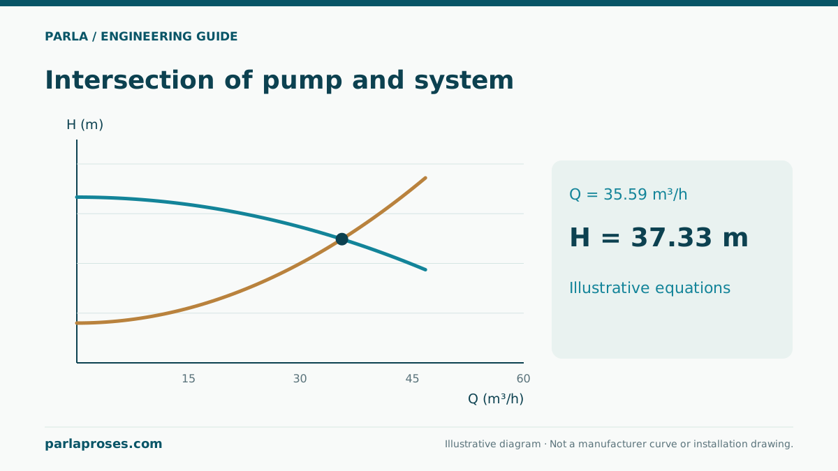
A centrifugal pump’s maximum catalogue flow is not the flow it will deliver in every installation. At a fixed speed, the pump curve shows the head available at each flow. The system curve describes the head needed to pass that flow through the installation. The steady duty point is the intersection where these two requirements match. Motor power or connection diameter alone therefore cannot establish the delivered flow.
The first decision is where the calculation begins and ends. Between two open tanks, the difference in free-surface elevations forms the static head. Transfer into a pressurised receiver also requires the surface-pressure difference. Surface velocities can be neglected in large tanks; if the boundaries are pipe sections with different velocities, include the velocity-head difference.
Build a system curve rather than a single design point
For turbulent flow of a low-viscosity liquid such as water, losses at a given valve position can often be approximated as proportional to Q². The resulting form is Hs = Hstatic + kQ². The coefficient k depends on the flow unit: inserting m³/s into a coefficient established for m³/h is incorrect. A more detailed calculation is needed if friction factor, valve characteristics or flow regime change substantially.
An installation with varying tank levels and valve positions does not have just one system curve. Separate curves for minimum and maximum levels allow the pump to be assessed across the actual operating range. Strainer fouling and the opening of parallel branches can also change the curve.
Worked example: solve the curve intersection
This illustrative example is not a manufacturer performance curve. With Q in m³/h and H in metres, assume a pump curve Hp = 50 − 0.01Q² and a system curve Hs = 12 + 0.02Q². Equating them gives 50 − 0.01Q² = 12 + 0.02Q², so Q² = 38/0.03. The positive root is Q = 35.59 m³/h; either curve then gives H = 37.33 m.
The table shows why 30 m³/h is not the natural duty point of this open system: at that flow the pump develops 11 m more head than the system requires. Unless valve position or speed changes, equilibrium occurs at a higher flow. At 40 m³/h, the pump head is insufficient.
| Flow Q | Pump Hp | System Hs | Interpretation |
|---|---|---|---|
| 0 m³/h | 50.00 m | 12.00 m | Mathematical origin; not a continuous operating point. |
| 20 m³/h | 46.00 m | 20.00 m | Pump head exceeds system demand. |
| 30 m³/h | 41.00 m | 30.00 m | The open system has not reached equilibrium. |
| 35.59 m³/h | 37.33 m | 37.33 m | Curve intersection; calculated duty point. |
| 40 m³/h | 34.00 m | 44.00 m | This pump cannot provide the required head under these conditions. |
Identify which curve a change affects
If the static head in the same example rises from 12 m to 18 m, the system curve shifts upward. The new equation is Q² = 32/0.03, producing a flow of 32.66 m³/h and a head of 39.33 m. The pump moves less water while operating at a higher head. This is a plausible result when the elevation difference between tanks increases.
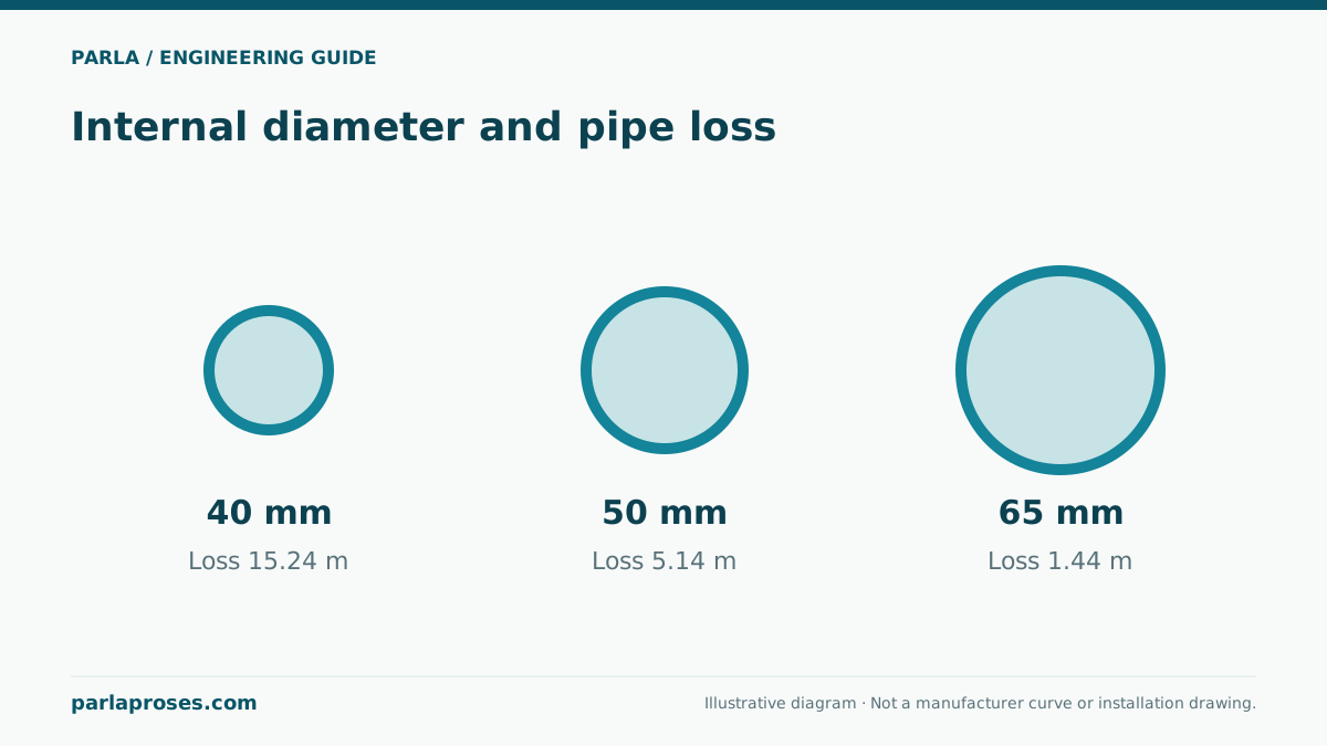
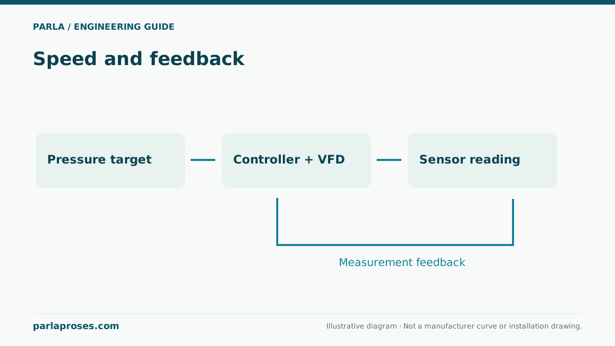
Throttling increases the resistance coefficient and steepens the system curve. A speed change instead alters the pump curve. Enlarging a pipe can reduce losses and increase flow with the same pump, so motor loading and suction conditions must be checked again after a diameter change. If the goal is simply to reduce flow, compare valve and speed-control options using the operating schedule and resulting energy consumption.
Selection checks continue after the intersection
Hydraulic equilibrium is only one step in selecting a suitable pump. The intersection must lie within the manufacturer’s permitted operating region for the selected impeller and speed. Check efficiency, NPSHr, motor loading and liquid properties at that same point. Maximum catalogue flow and maximum catalogue head cannot be combined into one simultaneous duty point.
Assuming a water density of 1000 kg/m³, the example hydraulic power from ρgQH is approximately 3.62 kW. If wire-to-water efficiency is assumed to be 65 percent solely for this calculation, input power is about 5.57 kW. This assumption is insufficient for selecting a motor rating: actual efficiency curves and shaft power across all permitted duty points are needed.
Compare the curve with commissioning measurements
Record flow, suction and discharge pressures, pump speed, tank levels and valve position at the same time. When calculating pump head from two pressure measurements, account for elevation and velocity differences between the measurement points. Do not immediately attribute low flow to pump failure: a closed valve, dirty strainer, air, incorrect speed or an omitted line resistance can produce similar results. Matching measured conditions to the calculation assumptions makes it easier to identify which curve has changed.
Frequently asked questions
Why does a 50 m pump produce 37.33 m in the example?+
The 50 m figure is the zero-flow value of the hypothetical curve. In this example, developed head falls as flow rises. Equilibrium with the installation occurs at 35.59 m³/h and 37.33 m; an actual selection requires a manufacturer curve.
Is the 12 m term constant at every flow?+
Yes in this example, because tank levels and surface pressures are fixed. If levels or receiver pressure vary, the static component changes too, and the curve must be updated for each relevant operating condition.
Does throttling make the pump produce less head?+
On the declining pump curve used here, throttling lowers flow while increasing the head developed at the duty point. Some additional head is lost across the valve. The actual change depends on curve shape and the control arrangement.
Does a calculated intersection prove that the selection is correct?+
No. Assess permitted flow range, efficiency, NPSH margin, power, materials and operating duration separately. A mathematically possible intersection may still fall outside the pump’s suitable continuous operating region.
Apply this assessment to your project.
Share your operating conditions, existing equipment and objective. Let’s assess product selection together with the technical documents.