Energy and controls
Variable-speed pump control: curve, sensor and limits
Slowing a pump does not deliver equal savings in every system. Assess static head, sensor placement, minimum flow and control stability together.
Illustrative engineering scenario · Assumptions are stated in the text.
AT A GLANCE
- Read affinity equations alongside the real system curve and fixed head.
- Record sensor, minimum speed, staging and fault behaviour at commissioning.
- Calculate savings from measured kWh and delivered service, not frequency percentage.
Separate changing and fixed head
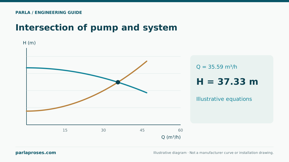
A variable-frequency drive changes motor frequency and, within its permissible range, pump speed, shifting the duty point. Keep static head, friction loss, valve behaviour and pump sequencing separate. A friction-dominated loop may use much less energy at lower speed; a large fixed elevation or required delivery pressure prevents assuming the same ratio. The affinity relations Q ∝ n, H ∝ n² and P ∝ n³ are approximations for comparable points on one pump. The real duty is the new intersection of pump and system curves.
A control project should therefore not promise “20% less speed means 49% less power” as a universal result. Assess pump efficiency, motor and drive losses, fixed head, control point and operating hours together. Friction often dominates a closed circulation loop, while static head can dominate a high-level supply.
Example: what does 40 Hz versus 50 Hz mean?
For a method-only example, assume 10 m³/h, 40 m and 5 kW pump shaft power at a comparable 50 Hz duty. If speed ratio n₂/n₁ = 40/50 = 0.8, approximate homologous values for the same pump are Q₂ ≈ 8 m³/h, H₂ ≈ 25.6 m and P₂ ≈ 2.56 kW. These are neither the measured duty in the target system nor an electricity-bill saving.
If the plant needs 30 m of fixed elevation and delivery-pressure head, 25.6 m at the homologous 40 Hz point falls short. The controller cannot simply stay at 40 Hz while maintaining the target; review the full pump curve and allowed operating range. In a friction-dominated loop, measured flow and electrical input can support a real savings estimate. Keep shaft power distinct from electrical input.
| Quantity | Assumed 50 Hz | Approximate 40 Hz | Limitation |
|---|---|---|---|
| Flow | 10 m³/h | 8 m³/h | Actual system intersection may differ |
| Head | 40 m | 25.6 m | Cannot meet 30 m fixed head |
| Shaft power | 5 kW | 2.56 kW | Not electrical input |
| Speed ratio | 1 | 0.8 | Check permitted speed range |
Sensor position changes the control objective
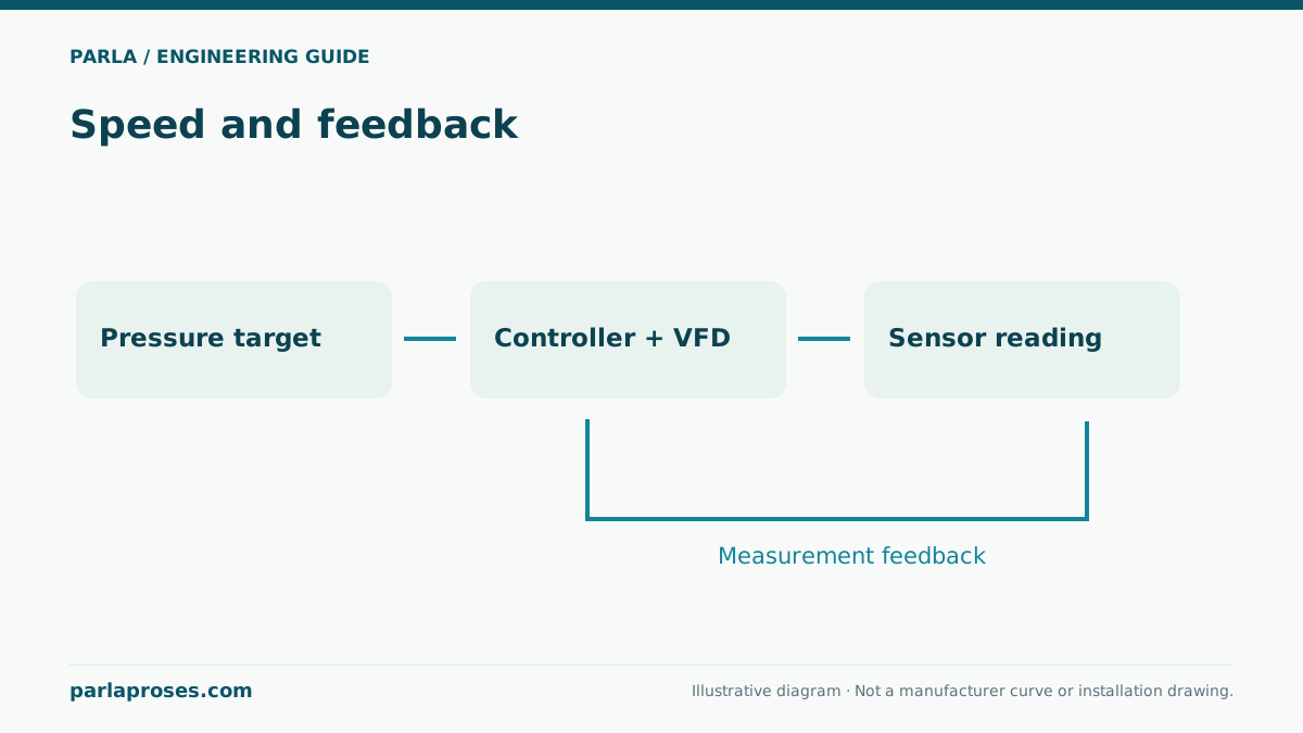
A sensor at pump discharge controls discharge pressure; it does not directly measure pressure at the remote critical consumer. As pipe losses vary with flow, check sensor location and setpoint across demand. For a remote sensor, specify communication-loss behaviour, calibration, redundancy and overpressure limits. A fast control loop is not always better: aggressive tuning can cause pressure hunting and frequent speed changes.
For a multipump booster, document lead-pump rotation, assistant-pump staging, low-flow sleep and minimum run-time logic. Check valves and pressure-vessel condition can affect stability. During commissioning simulate low, typical and high demand and log remote pressure, electrical input and frequency together.
Record electrical and maintenance limits
Select the drive within motor and pump limits, supply quality and environmental conditions. Check cable length, insulation, filters and electromagnetic compatibility to the project requirements. Some applications require a prohibited resonance band; establish it from measurements and manufacturer data. Frequency display alone proves neither delivered pressure nor actual energy use.
Log flow, pressure, frequency, kW and operating hours over the baseline. Compare periods at equivalent service levels later; do not report an energy percentage without adjusting for production and weather changes. The control objective is stable pressure and process service. Economic benefit is verified through measured energy and maintenance outcomes.
Frequently asked questions
Does power always fall 49% at 40 Hz?+
No. 0.8³ is an approximate shaft-power affinity result. Static head, actual duty, efficiencies and drive losses change electrical input.
Must the pressure sensor always be at discharge?+
No. Choose the control point from critical service needs and define communication and fail-safe behaviour for a remote sensor.
How do we set minimum frequency?+
Check manufacturer speed, minimum flow, cooling and required process pressure; there is no universal value.
Does installing a drive guarantee energy savings?+
No. It depends on system curve and control logic meeting the demand profile. Measure savings over comparable periods delivering the same service.
Apply this assessment to your project.
Share your operating conditions, existing equipment and objective. Let’s assess product selection together with the technical documents.